
 0


A simplified illustration of the resolving of a domain name is in the following picture, where we ask a name server of each level just once. In a more real-life scenario, the number of steps is even greater due to redirections using CNAMEs and DNAMEs, the need for the DNSSEC signatures of the records, to be able to validate them, etc.
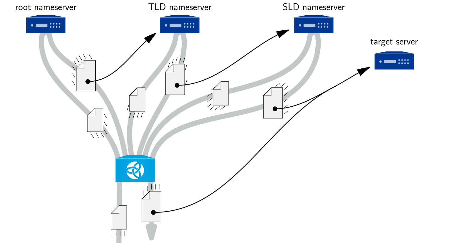
When we get an answer from an authoritative server, we insert it into the cache. But since the size of the cache is limited, we may need to evict some records from time to time and this is where the need for the garbage collector arise. It periodically checks the cache utilization and if it is over the set limit the whole cache is scanned and some percent of the stored records is removed. Crucial here is to know which records are worth to be kept in the cache.
What would be even better is to ask authoritative servers in advance for the records which will be needed in the future. There may be different approaches how to guess which records are the right ones based on the past queries, their timings, etc. We currently stick to a more conservative prefetch mechanism, which only updates some records shortly before their expiration. We can guarantee that our traffic to the upstream will not rise significantly and this guarantee is per record — i.e. we limit the number of extra requests to the upstream by a fraction of client queries that needed the record. We also try not to increase the used space by updating only records which are already stored in the cache, although new intermediate records may still appear as a side effect.
The main and common part of both garbage collector and prefetch is how to determine which records are useful enough to be kept in the cache or even updated; and this is the part which was rewritten. Both mechanisms were already present in the previous versions, but overall they were too simple.
The current classification of the usefulness of records is based on our KRU data structure, which we originally introduced as part of our DoS protection article and then thoroughly described in the follow-up technical solution article. This time, we use KRU for counting the accesses to the individual cache records so that we can compare how frequently they were used recently.
We first recap basic properties of KRU. Then we describe garbage collector in more detail comparing its old and new version and support the improvement with the measurements. After that, we present our new prefetch mechanism along with a brief note about its precursors and again show a chart of the experimental comparison. Finally, we comment on possible clashes between the garbage collector and prefetch and provide some recommendations on their configuration.
The KRU-based garbage collector is already present in Knot Resolver since v6.0.17, the new prefetch mechanism will be present in the next release v6.6.0.
Comparing the usefulness by KRU
In a nutshell, the Knot Recently Used data structure stores counters, which can be effectively incremented and their values read. As time passes, the values of the counters are continuously decreasing by so called exponential decay, so rather than counts they represent recent frequencies of the tracked events. See the articles referenced from the introduction for details.
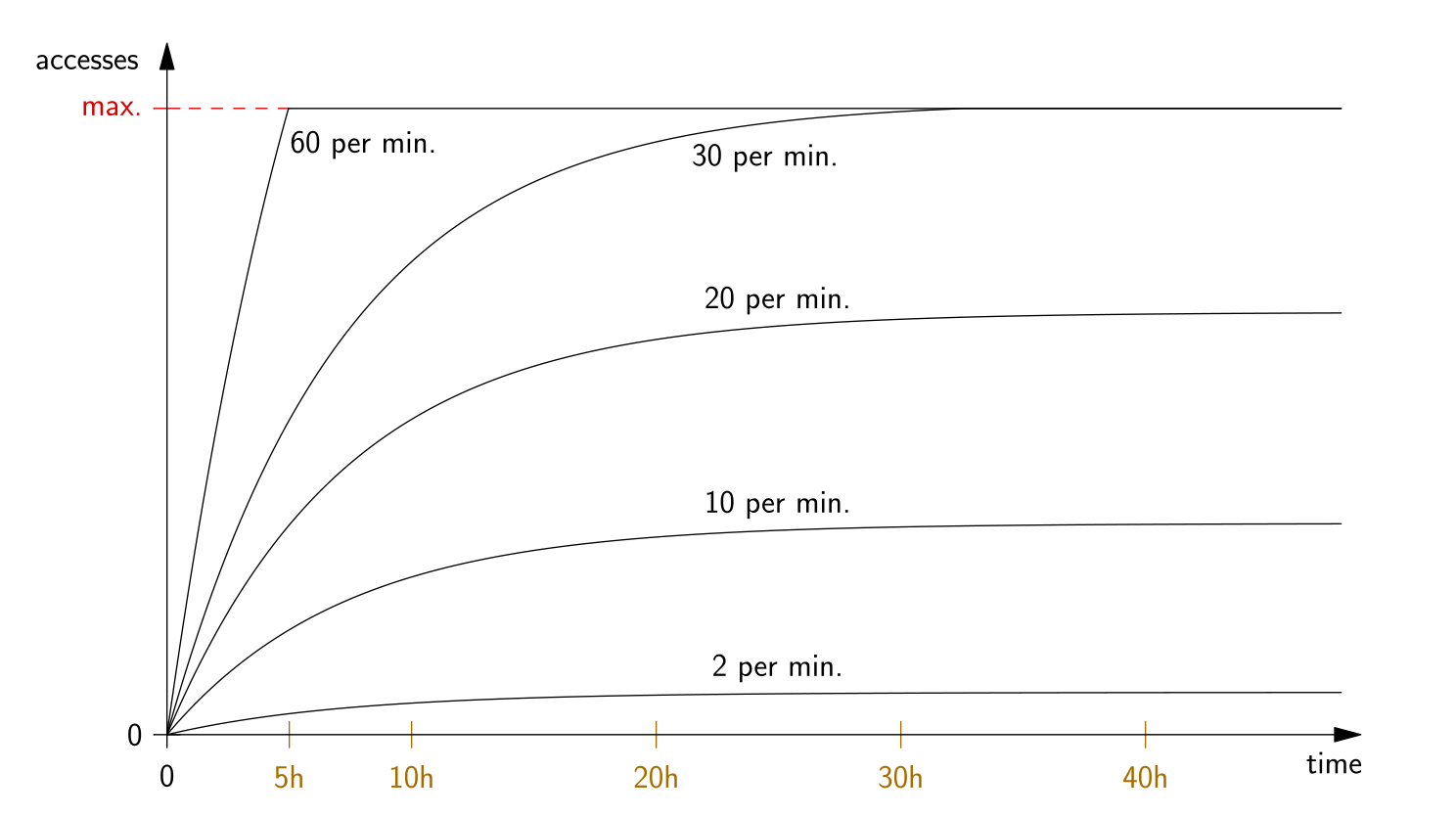
In this case, we count accesses to the individual records stored in the cache and the values are halved in 5h by multiplying with a constant slightly less than one each second. The precision of the counters then implies that the individual increments are fully forgotten after 80 hours. If the accesses to a record are regular, the combination of linear increase and exponential decay tends to an equilibrium around a value proportional to the access rate, as can be seen on the following chart. The greater the values are the more useful the record is considered.
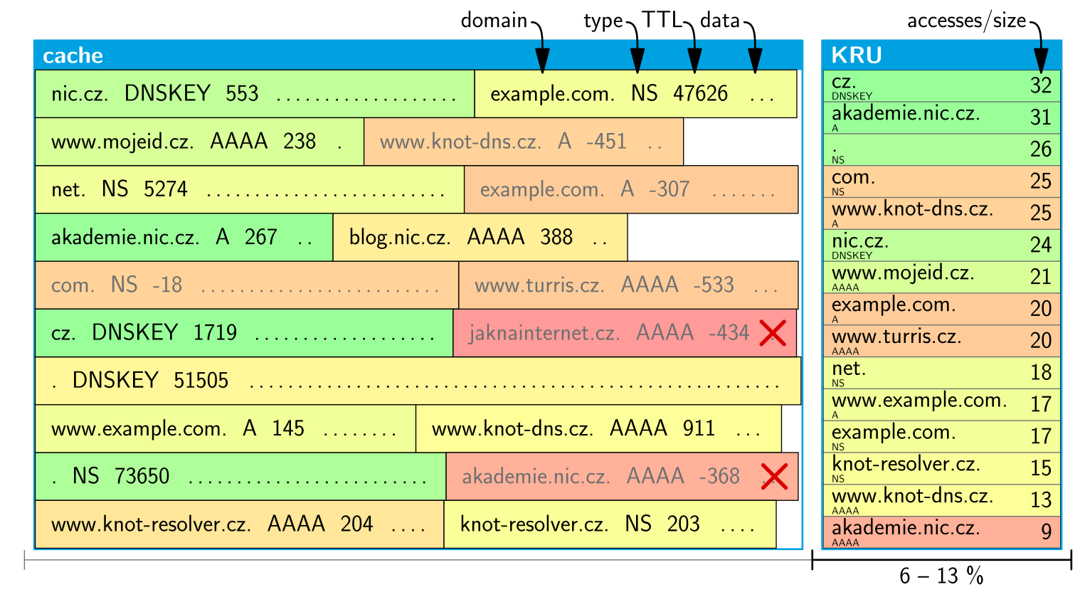
The size of KRU is constant and has to be rounded to a power of two — we have chosen it to be 6–13 % of the configured size of the cache and the actual cache data storage is lowered by this amount.
There is no synchronization between keys stored in cache and those having their counters in KRU. It is possible that a record is evicted from cache, because it expired, but still has a large value in KRU. And on the other hand, the counter value of the key may get zeroed, while the record is kept in the cache, because there was no need for evictions. Furthermore, from the KRU design it is not even possible to say that a key is not present there — the counters with too low values just merge together and new keys may take the shared values over while getting popular.
To be more precise, we use a little different metrics in GC and in prefetch. For garbage collector, the space in cache is the limited resource, so we are in fact interested in access rate per byte of the cache — the increments are thus divided by the size of the corresponding records. The greater the record is the more accesses are needed not to evict it. In other words, there is no difference between one record with some number of accesses and two half-sized records with half of the number of accesses each. The upper bound of one access per two seconds, above which the access frequencies are indistinguishable in the chart above, is related to records of a normal size defined by us. In prefetch, we use the same instance of KRU, but multiply the read counts back by the sizes of the records as space is not relevant there.
Garbage Collector
The garbage collector of the Knot Resolver is a separate process spawned alongside the kresd processes. In a default configuration, it checks the cache utilization every second, and if it exceeds 80%, the content of the cache is analysed and 10% of the used space is freed. All three parameters are configurable along with the cache size.
The analysis consists of two linear scans of all the records stored in the cache. In the first pass, we assign an integer category number (0–99) to each of them with lower categories being considered more useful and compute the space occupied by records in each category. Then we incrementally sum up the sizes from highest categories to determine the limit category number separating the ones for retaining and removal. Finally, we perform the second scan, categorizing everything again and removing the records with too high category number.
Up to this point, there is almost no change between the versions. Just the categorization itself was rewritten completely.
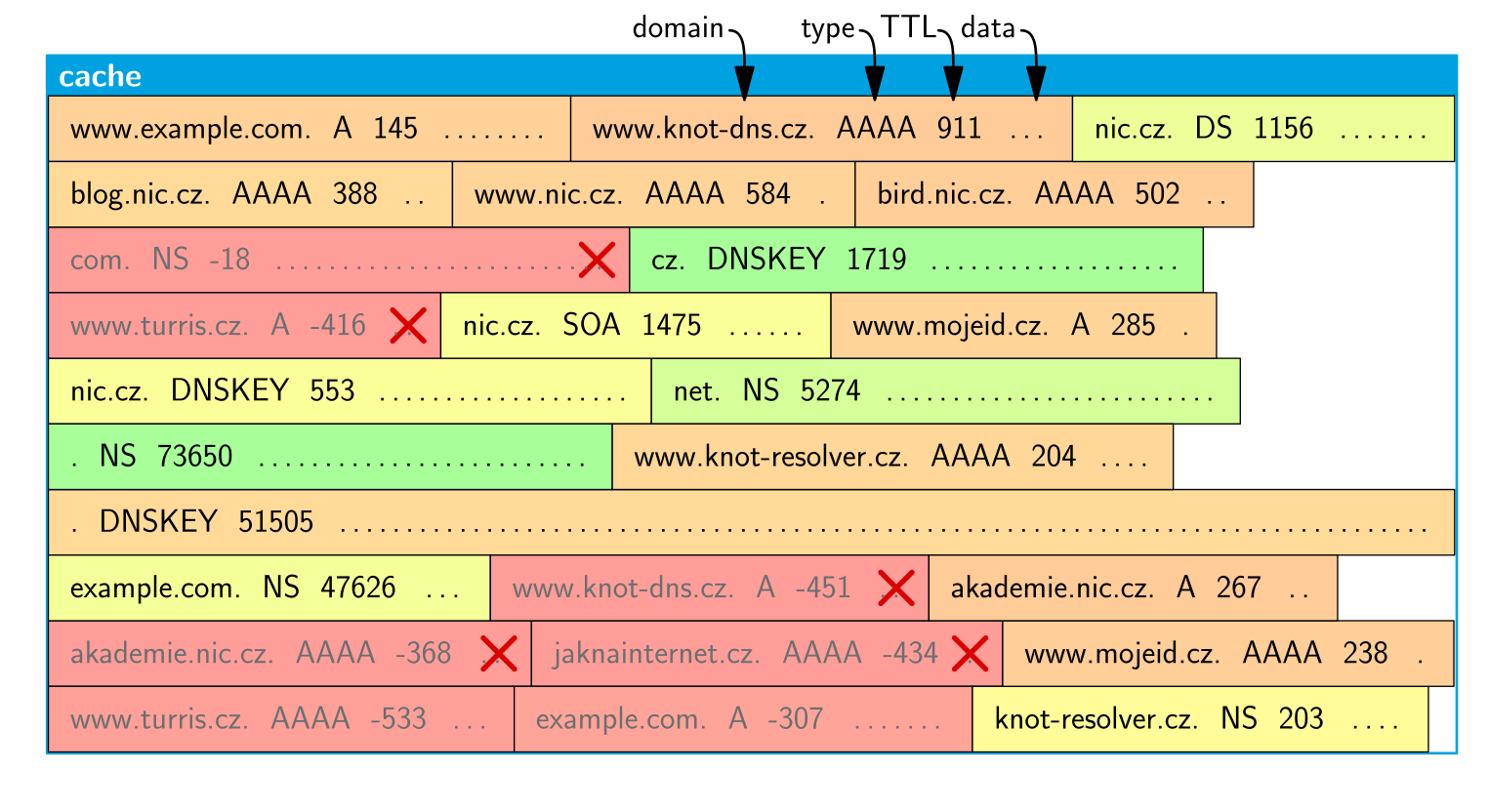
Originally, no information about accesses was stored and so only the actual data of resource records had to be used for deciding. The main partitioning was into groups of expired records, valid 3rd and lower levels domain records, valid SLD, valid TLD+root. Minor criteria were based on record type, whether it is oversized, and some randomness. Typically, it thus removed first all the expired records and then third and lower level domains irrespective of their actual popularity. See the example categorization (from green to red) in the following image.
As we mentioned in the previous section, we lowered the size of the database part of the cache to store KRU usage statistics beside it. Having those data, categorization turns out to be pretty simple. Our primary criterion is whether the record is expired, dividing the categories into halves, and the secondary criterion is the access frequency per byte stored in the KRU, partitioning the halves much smoother even than originally. See the next image.
Measurements
To see the improved behaviour on the real traffic, we need as long traffic data as possible, so that KRU statistics become relevant. We intentionally use small cache size to emphasize garbage collector decisions. On the other hand, we don’t need high load here. In particular, the traffic recording had 9 hours and 2000 QPS and the cache size was 25 MB. We compare it with the behaviour of 40 GB cache, where no GC is needed at all and so it is the best where we can get.
As the latency of resolving differs significantly based on how many of the required authoritative answers are cached, we use the latency as the measure to compare the implementations. In the following logarithmic percentile histogram of the latencies, you can see that KRU-based GC is much closer to the large cache than the original simple GC.
To get a better idea of how to interpret the chart, imagine that you have all the measured response times on individual queries on vertical axis and order them from the highest ones to lowest, left to right, drawing a line through them. If the latencies are lower, the line will be lower; if there is a lower number of high-latency responses, the corresponding part of the line moves to the left; both cases signify better results. Finally, both axes are logarithmic to emphasize the number of high-latency responses but keep mutually comparable the ones which are by orders of magnitude faster.
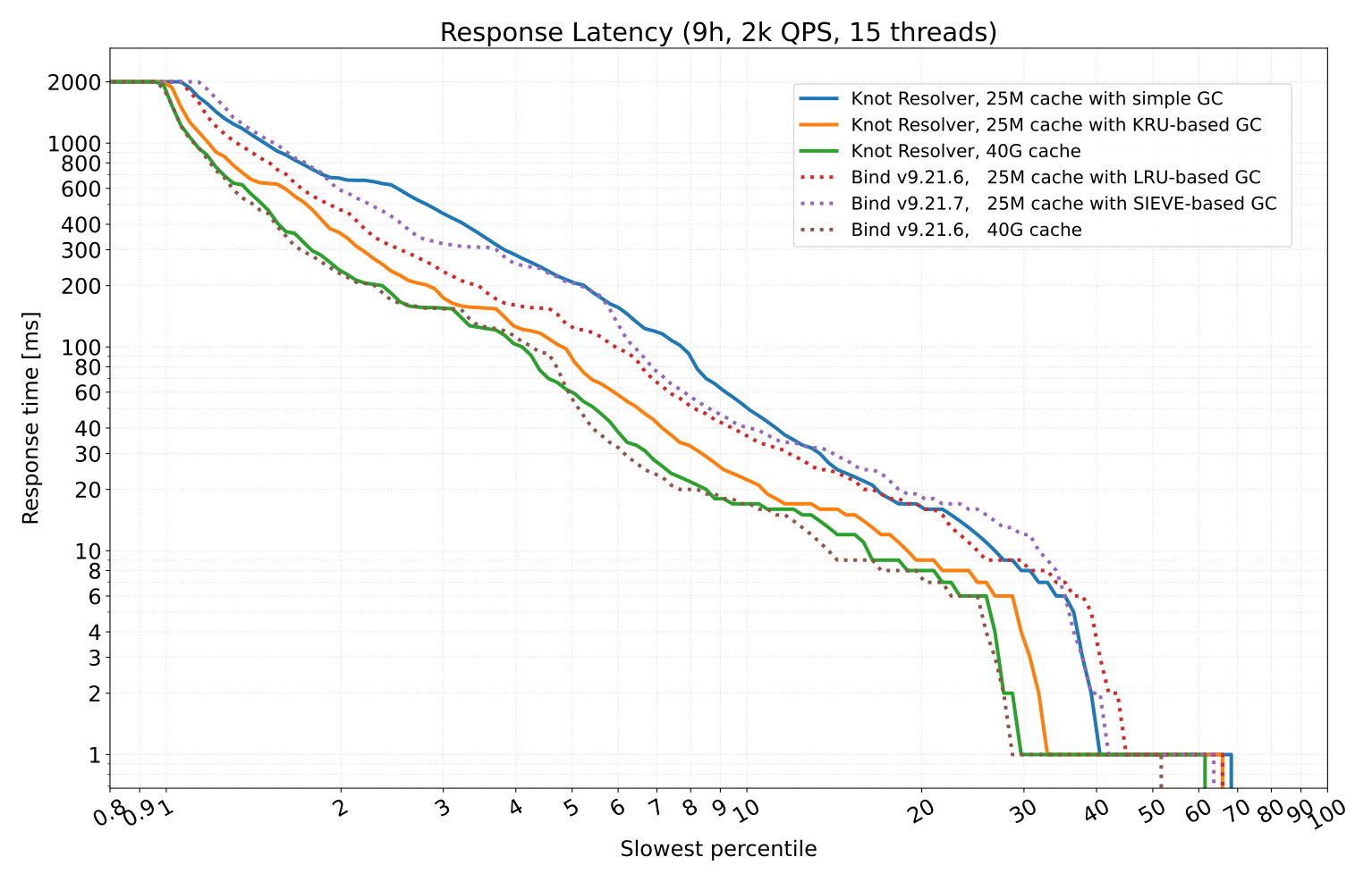
We also measured BIND 9 the same way, drawn with dotted lines in the chart, and our KRU-based GC seems to perform better in this scenario. A little unexpected result is that their newer SIEVE-based GC seems to be a little worse than the original LRU-based; it however doesn’t contradict their measurements with opposite outcomes as their number of QPS was much higher. Their goal was to increase throughput by avoiding locking in LRU implementation instead of improving what to evict. Our KRU-based statistics are lock-free by design, but high-load comparison was not included in our measurements.
Prefetch
Originally, we used prefetch and predict Lua modules. The former allows refreshing records which were asked for shortly before their expiration; it statistically works but we can now do better with KRU. The latter was trying to learn usage patterns and was appointed as experimental and not recommended for production use at all. Both of them are now considered obsolete and are not available from YAML configuration; they can still be activated from Lua if needed.
Our new prefetch mechanism is written purely in C and adopts the YAML configuration tree of the old one extended by further optional settings. In particular, we can configure the guarantee restricting the increase in traffic to upstream related to the number of client queries. We can also limit the updated records by their access rate and adjust how long before expiration the update may occur.
As said above, we can calculate the access rate to a record from the value of its counter in KRU under the assumption that the accesses are regular. This is, however, not enough for the guarantee that we want to provide. Instead, we want to be sure that at least the configured number of accesses, let’s call it k, were performed to allow the update and that we will not count them again later.
We thus need the counter value to be so high that decay will decrease it by k by the time we will be considering it’s next update. This matches the worst case where all k accesses occur just before reading the value; for regular accesses the requirement turns out to be more strict. It may be the case that other accesses will in fact cancel the effect of decay, but this is not an issue here, because we just read the value once and consider its awaited decrease. On the other hand, if further accesses keep the value high, we can repeat the reasoning for the next update with different k accesses considered.
Now, it would be straightforward to read the value just before possibly performing the update and decide whether it will decrease enough before the updated record expires — but we don’t know yet what will be its new TTL. Instead, we consider the counter value just after getting the record from upstream, and if it is high enough, we schedule the update to occur shortly before expiration. To be precise, we consider the time period between receiving the record from upstream and the point to which its update would be scheduled, which is at least 5s before the expiration. The actual update then occurs the earliest after that point when a kresd process gets idle.
See the procedure in the next image. The horizontal axis is the time arrow. The green rectangles inside it are the validity periods of possibly different versions of the single given cache record and the orange periods before them signify obtaining them from upstream. Relevant client queries and corresponding answers are shown under the time arrow and the evolution of the corresponding KRU counter value is the sawtoothed line above it. We see that receiving the record on user request initiated the scheduling process, creating a plan when the update may occur. The actual update is initiated a little bit later and after receiving the updated record a new scheduling is initiated.
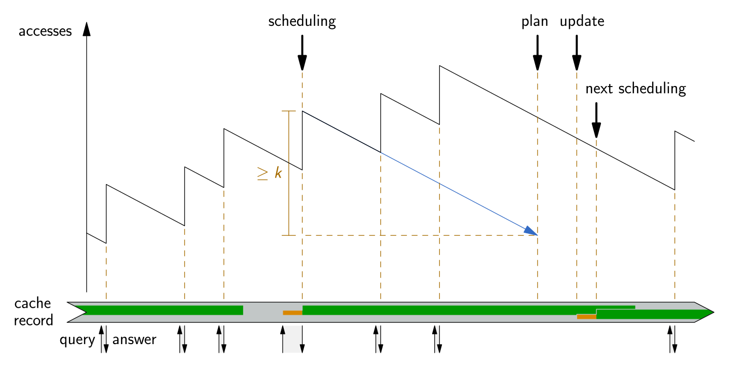
Similarly, we add the requirement for the minimal access rate, or more precisely maximum access period. Here, we require the counter decrease of at least one per the set access period. We note that there is a difference between one access by some time and two accesses by double time, because of how the exponential decay works, — for the same reason we consider period more precise than frequency here.
Both requirements result in the lower bounds on the counter value and based on the TTL of the specific record one may be stricter or the other, so we take the higher of them. The bound has to be met both at the time of scheduling and just before the update to initiate it. To meet the guarantee, the former test is sufficient, but intuitively the popularity closer to the update seems even more important. For the second condition, it would be even better if it is met for the whole validity period of the record, but due to a technical reasons we test it only twice.
We said that the update is scheduled at least 5s before the expiration. It can be configured to be some percent of TTL, by default 1 %, but still at least those 5s. By increasing the value, we can avoid short TTL of useful cached records, which can help caching clients to avoid repetitive queries and so decrease our traffic to them. On the other hand, it also shortens the time between getting the record and its following prefetch, thus making the guarantee condition more strict and increasing number of our queries to upstream for the still prefetchable records.
If there is no time to initiate the update even 2s before the expiration, the calculated bound for access frequency starts rising till the time of expiration when the prefetch is cancelled. This way, we try to choose the more useful records out of those already selected in case we don’t have enough time to update them all. We also don’t want to delay prefetching after expiration not to cascade the delays much for other records.
We remark that using the prefetch along with forwarding mode will probably not work well, because the update before the expiration will likely get the same record from the other resolver incl. its short remaining TTL.
Measurements
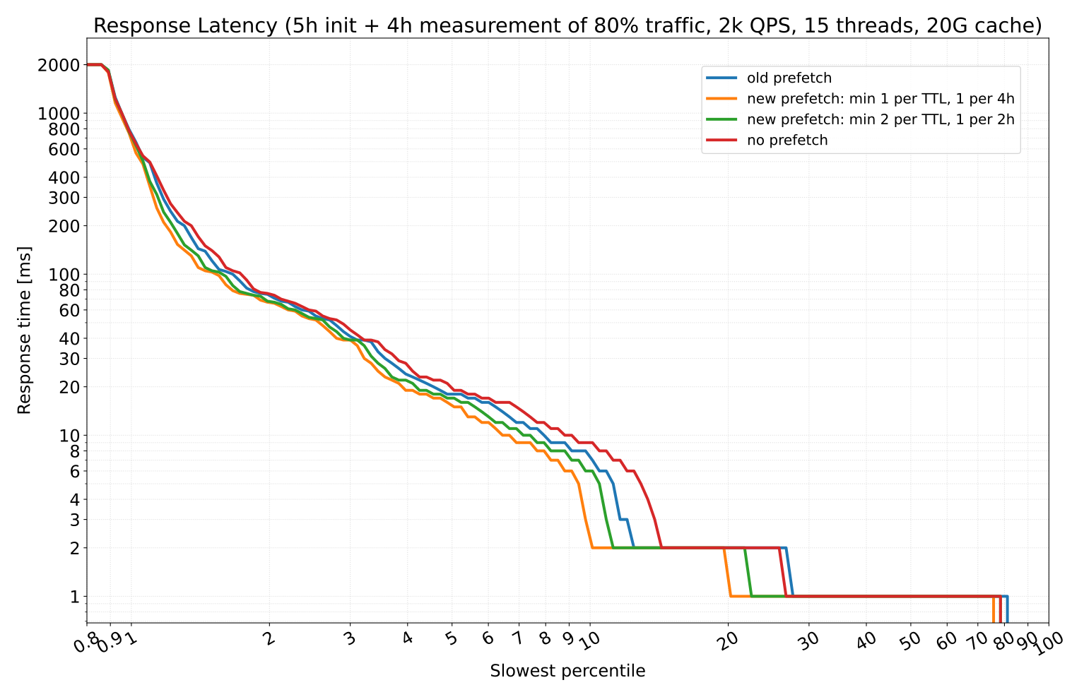
As in the case of GC, we performed experimental measurements to demonstrate the improvement. This time, we used large cache so that records stay in cache until their expirations and prefetching may get involved.
We also divided the replaying of the traffic into two phases: we use the first 5h to just sum up some values in KRU and only the remaining 4h are counted in the resulting chart. The reason for this is that here we compare the values to the threshold based on the configuration, while in GC we compared the values just to each other and so having them proportionally smaller wasn’t an issue. After those 5 hours, and again with regular accesses, the values in the counters are supposed to be half in comparison with a long-term running resolver. We can therefore expect that the real behaviour with some configuration will be somewhere between the measured one with that configuration and with two times weaker thresholds.
The last change is that we tracked only 80 % of the traffic with the most repetitive queries to be included in the chart to emphasize the different behaviour between the variants. The low-repetitive queries will probably not incur any prefetching, so almost no difference in latency is expected for them. Based on the data, the chosen queries have minimum average frequency of one query per 30 minutes and contain only 1/8 of the unique queries.
In the following chart, you can see the comparison of using no prefetch, old prefetch (but no predict) and different configurations of the new prefetch. The default configuration is represented by the green curve, but we expect its long-term behaviour closer to the yellow one from the reasons above. Both of them perform better than no prefetch and old prefetch.
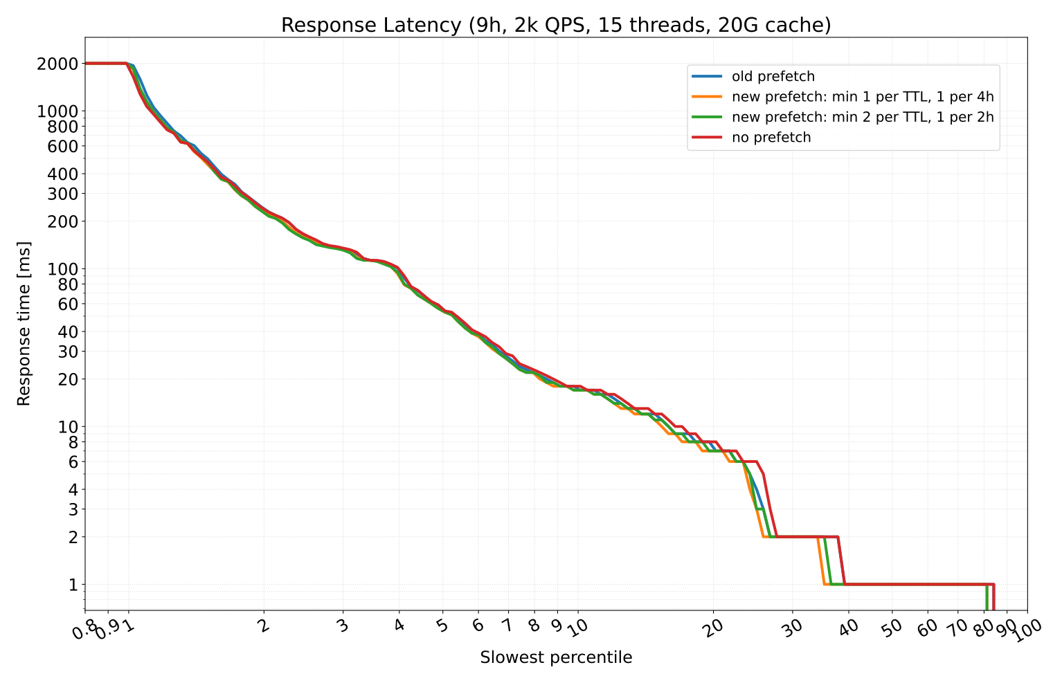
We also performed a measurement with all queries tracked, i.e. whole 9h and incl. the low-repetitive ones. As you can see in the following chart, the improvement is still noticeable, but not much significant in this setting, which was expected.
Cache configuration and GC statistics
It might have been difficult to find out even the optimal size of the cache. With prefetch, new configuration options arose, and as garbage collector and prefetch have in some sense opposite goals, misconfiguration may lead to clashes. To provide a clue how to configure it, we added detailed statistics of what is being removed during garbage collection, so that you can recognize possible issues.
The basic advice for setting the cache size is as follows. For personal use and small offices several tens of MB may be sufficient, use 100 MB if there is no pressure. For large dedicated deployments, you may utilize even gigabytes of cache, but keep in mind that the whole cache still has to fit into RAM, even if it is stored on disk, to avoid page misses and subsequent performance issues. You have to keep some memory for OS, local data and at least 50-100 MB for each worker based on the load — this applies to mostly UDP traffic and version 6.5.0 with significantly lower memory footprint of workers than in previous versions. As the memory consumption of workers rises under high load, keep the margin higher and start with smaller cache. If garbage collection runs only rarely, the chosen size is probably sufficient. Otherwise check the output of the garbage collector.
You can find the following lines in the log after each garbage collection, i.e. after exceeding the configured cache utilization limit. You can also run GC process manually, possibly as dry run with modified settings, to analyze cache content on demand.
Canceling prefetch for
      #.## MB of kept valid RRs eligible for prefetch (limit category #),
      #.## MB of expired RRs (not updated in time, incl. those for removal);
removing (limit category #)
      #.## MB /     #.## MB of valid RRs eligible for prefetch,
      #.## MB /     #.## MB of other valid RRs,
      #.## MB /     #.## MB of expired RRs,
      #.## MB /     #.## MB of RTT entries,
      #.## MB /     #.## MB of prefetch entries (incl. cancellation),
      #.## MB /     #.## MB (# records) in total.
Besides resource records, cache contains round-trip time entries allowing comparisons of latencies of alternative authoritative servers and newly also prefetch entries serving as time-ordered pointers to RRs planned for update.
Ideally, we would like to remove only expired RRs, which are not much useful anymore, unless serving stale answers. Removing valid RRs may be suboptimal if they are needed in the future, but we still first remove the less useful ones, so removing some fraction of them may be also healthy. If the fraction is higher, consider increasing the cache size.
The real issue is if we are removing valid RRs which are eligible for prefetch, i.e. they passed the conditions at insertion and still meet the computed lower bound on accesses. In this case, we need either to increase the cache size or make the prefetch conditions more strict, not to update so many records. Prefetch is always used only for records which are already present in the cache, so removing those entries also cancels their prefetching; after obtaining them the next time, their prefetch may be however scheduled again.
We may be cautious even if GC cancels scheduled prefetch for valid RRs which are not yet being removed. In the default settings, GC frees up 10 % of the occupied capacity and for another 10 % prefetch is cancelled. This serves as a buffer between records for prefetching and records for removal, which helps mitigating the clashes. We however still recommend to adjust the settings if this happens.
Another warning arises from canceling prefetch of expired RRs. This means that kresd processes had not enough cpu time to initiate update of those RRs within the configured time period before their expiration. If this happens, kresd normally removes those prefetch entries by itself immediately after entering the prefetch stage when idle, which also wasn’t the case. If you are under DoS attack, this is correct behavior: client requests will be prioritized according to what seems to be legitimate traffic, some queries of the attacker may be dropped and prefetch will not be used at all. If this happens repeatedly under normal load, make prefetch conditions more strict or examine whether the overall performance is sufficient. These prefetch entries may also be a relict after disabling prefetch, in which case kresd just ignores them, or after some period of not running the resolver at all.